python opengl draw 3d scatter plot

Scatter plot is a graph in which the values of 2 variables are plotted along two axes. Information technology is a almost basic type of plot that helps you visualize the human relationship between two variables.

Concept

1. What is a Scatter plot?
2. Basic Scatter plot in python
3. Correlation with Scatter plot
4. Changing the colour of groups of points
5. Changing the Colour and Marking
6. Besprinkle plot with Linear fit plot using seaborn
7. Scatter Plot with Histograms using seaborn
8. Bubble plot
9. Exploratory Assay using mtcars Dataset
   • Multiple line of best fits
   • Adjusting colour and style for unlike categories
   • Text Annotation in Scatter Plot
   • Bubble Plot with categorical variables
   • Categorical Plot

What is a Scatter plot?

Scatter plot is a graph of 2 sets of information along the two axes. It is used to visualize the human relationship between the ii variables.

If the value along the Y axis seem to increase as 10 axis increases(or decreases), information technology could indicate a positive (or negative) linear relationship. Whereas, if the points are randomly distributed with no obvious pattern, it could possibly signal a lack of dependent relationship.

In python matplotlib, the scatterplot tin be created using the pyplot.plot() or the pyplot.scatter(). Using these functions, you can add more than feature to your besprinkle plot, like irresolute the size, colour or shape of the points.

So what is the difference between plt.besprinkle() vs plt.plot()?

The deviation between the two functions is: with pyplot.plot() whatever property you utilise (color, shape, size of points) will be applied across all points whereas in pyplot.scatter() you accept more control in each indicate'south appearance.

That is, in plt.besprinkle() yous tin can have the color, shape and size of each dot (datapoint) to vary based on another variable. Or even the aforementioned variable (y). Whereas, with pyplot.plot(), the properties you ready will be practical to all the points in the chart.

First, I am going to import the libraries I volition be using.

                      import            pandas            every bit            pd            import            numpy            every bit            np            import            matplotlib.pyplot            equally            plt %matplotlib inline plt.rcParams.update({'figure.figsize':(ten,8),            'effigy.dpi':100})                  

The plt.rcParams.update() office is used to modify the default parameters of the plot'southward figure.

Basic Scatter plot in python

First, let'southward create artifical data using the np.random.randint(). You need to specify the no. of points yous require equally the arguments.

You lot can also specify the lower and upper limit of the random variable y'all need.

Then use the plt.besprinkle() function to draw a scatter plot using matplotlib. You demand to specify the variables x and y as arguments.

plt.championship() is used to prepare championship to your plot.

plt.xlabel() is used to label the ten axis.

plt.ylabel() is used to label the y axis.

          #            Simple            Scatterplot            x = range(50) y = range(50) + np.random.randint(0,thirty,l) plt.scatter(10, y) plt.rcParams.update({'effigy.figsize':(10,viii),            'effigy.dpi':100}) plt.title('Simple            Scatter            plot') plt.xlabel('Ten            - value') plt.ylabel('Y            - value') plt.evidence()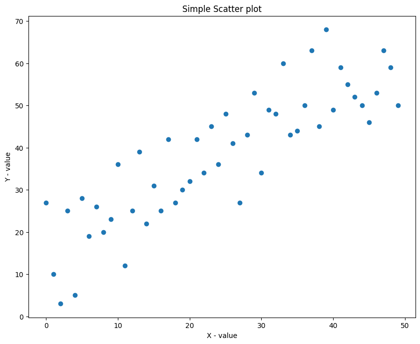                  

You tin can see that there is a positive linear relation between the points. That is, as Ten increases, Y increases as well, because the Y is really only 10 + random_number.

If you want the color of the points to vary depending on the value of Y (or another variable of aforementioned size), specify the colour each dot should accept using the c argument.

You can also provide unlike variable of same size as X.

          #            Uncomplicated            Scatterplot            with            colored points ten = range(fifty) y = range(50) + np.random.randint(0,30,50) plt.rcParams.update({'figure.figsize':(10,8),            'figure.dpi':100}) plt.scatter(x, y, c=y, cmap='Spectral') plt.colorbar()            plt.championship('Simple            Scatter            plot') plt.xlabel('10            - value') plt.ylabel('Y            - value') plt.show()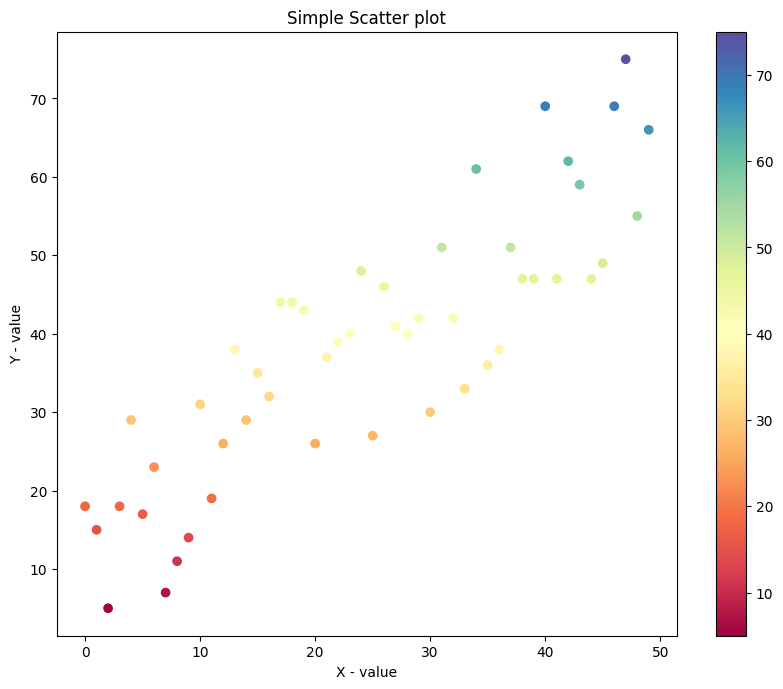                  

Lets create a dataset with exponentially increasing relation and visualize the plot.

          #            Scatterplot            of            not-random vzriables x=np.arange(1,x,0.2) y= np.exp(ten) plt.besprinkle(x,y) plt.rcParams.update({'figure.figsize':(x,8),            'figure.dpi':100}) plt.title('Exponential            Relation            dataset') plt.show()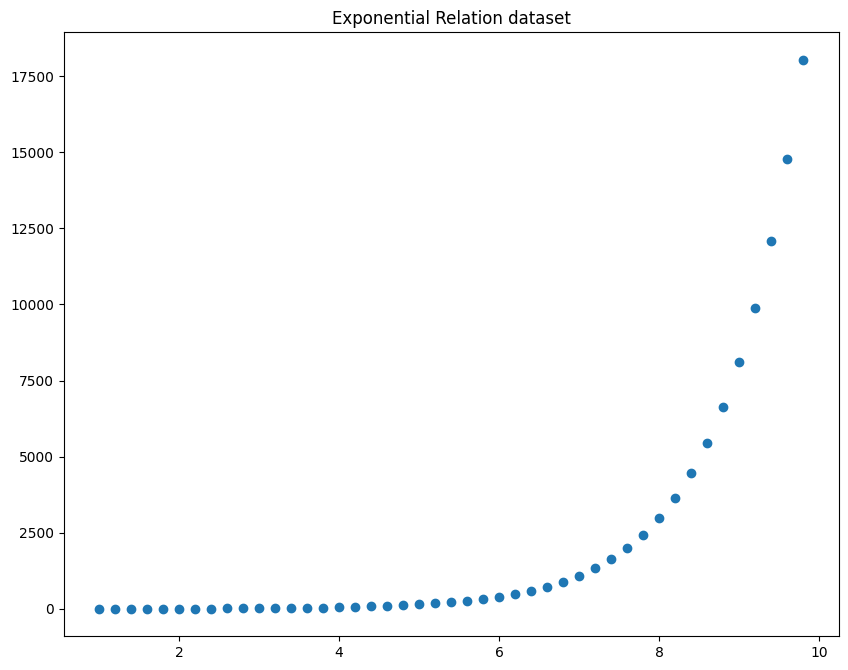                  

np.arrange(lower_limit, upper_limit, interval) is used to create a dataset between the lower limit and upper limit with a footstep of 'interval' no. of points.

Now you can see that there is a exponential relation between the x and y centrality.

Correlation with Scatter plot

one) If the value of y increases with the value of x, then we tin can say that the variables have a positive correlation.

2) If the value of y decreases with the value of x, then we can say that the variables take a negative correlation.

iii) If the value of y changes randomly independent of x, then it is said to take a nothing corelation.

          # Scatterplot            and            Correlations # Data x=np.random.randn(100) y1= 10*v            +9            y2= -five*ten y3=np.random.randn(100)  # Plot plt.rcParams.update({'figure.figsize':(x,eight), 'figure.dpi':100}) plt.scatter(x, y1,            label=f'y1 Correlation = {np.round(np.corrcoef(x,y1)[0,ane],            2)}') plt.besprinkle(x, y2,            label=f'y2 Correlation = {np.round(np.corrcoef(x,y2)[0,i],            2)}') plt.scatter(x, y3,            label=f'y3 Correlation = {np.round(np.corrcoef(x,y3)[0,1],            2)}')  # Plot plt.title('Scatterplot            and            Correlations') plt.legend() plt.show()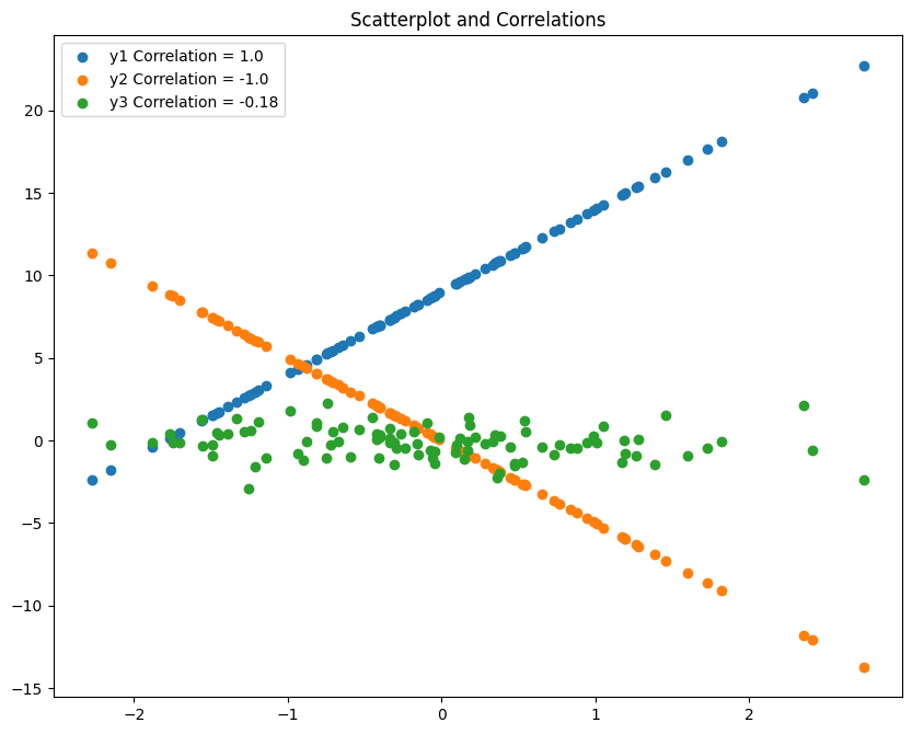                  

In the above graph, you tin can encounter that the blue line shows an positive correlation, the orange line shows a negative corealtion and the green dots show no relation with the x values(it changes randomly independently).

Changing the color of groups of points

Use the color ='____' command to change the colour to correspond besprinkle plot.

                      # Scatterplot - Colour Change            x = np.random.randn(50) y1 = np.random.randn(fifty) y2= np.random.randn(50)            # Plot            plt.scatter(x,y1,color='blue') plt.besprinkle(x,y2,color=            'red') plt.rcParams.update({'figure.figsize':(x,viii),            'figure.dpi':100})            # Decorate            plt.title('Colour Change') plt.xlabel('X - value') plt.ylabel('Y - value') plt.show()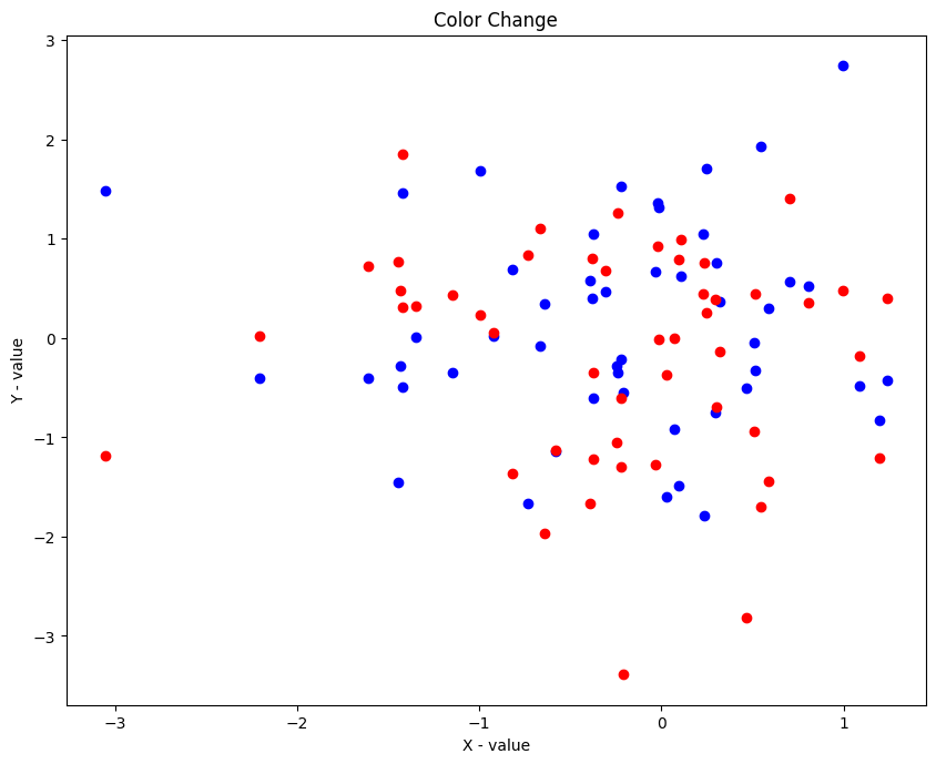                  

Irresolute the Colour and Marking

Apply the marking =_____ control to alter the marker type in scatter plot.

['.','o','v','^','>','<','southward','p','*','h','H','D','d','1′,","] – These are the types of markers that you can utilize for your plot.

                      # Scatterplot of dissimilar distributions. Color and Shape of Points.            x = np.random.randn(500) y1 = np.random.randn(500) y2 = np.random.chisquare(x,            500) y3 = np.random.poisson(5,            500)  # Plot plt.rcParams.update({'figure.figsize':(10,viii),            'effigy.dpi':100}) plt.scatter(x,y1,colour='blue', marking=            '*',            label            ='Standard Normal')            plt.besprinkle(10,y2,color=            'reddish', marker='v',            characterization            ='Chi-Square')            plt.scatter(ten,y3,color=            'green', marker='.',            characterization            ='Poisson')                        # Decorate plt.title('Distributions: Colour and Shape change') plt.xlabel('10 - value') plt.ylabel('Y - value') plt.legend(loc='best') plt.show()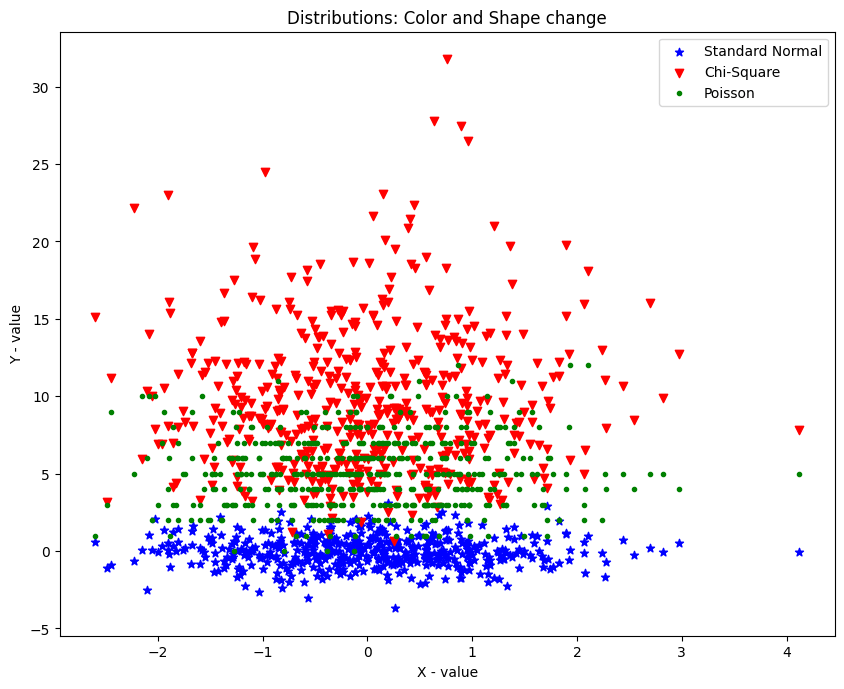                  

Scatter Plot with Linear fit plot using Seaborn

Lets try to fit the dataset for the best fitting line using the lmplot() function in seaborn.

Lets utilize the mtcars dataset.

You can download the dataset from the given address: https://www.kaggle.com/ruiromanini/mtcars/download

Now lets try whether there is a linear fit between the mpg and the displ column .

          # Linear - Line of all-time fit            import            seaborn            as            sns url =            'https://gist.githubusercontent.com/seankross/a412dfbd88b3db70b74b/raw/5f23f993cd87c283ce766e7ac6b329ee7cc2e1d1/mtcars.csv'            df=pd.read_csv(url) plt.rcParams.update({'figure.figsize':(10,8),            'figure.dpi':100}) sns.lmplot(x='mpg', y='disp',            information=df) plt.title("Scatter Plot with Linear fit");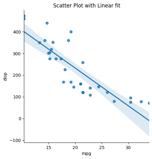                  

You tin encounter that we are getting a negative corelation between the 2 columns.

          #            Scatter            Plot            with            lowess            line            fit            url = 'https://gist.githubusercontent.com/seankross/a412dfbd88b3db70b74b/raw/5f23f993cd87c283ce766e7ac6b329ee7cc2e1d1/mtcars.csv'            df=pd.read_csv(url) sns.lmplot(x='mpg', y='disp', data=df,            lowess=Truthful)  plt.title("Scatter Plot with Lowess fit");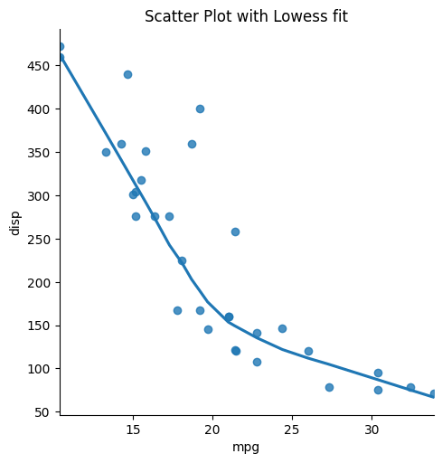                  

Scatter Plot with Histograms using seaborn

Use the articulation plot function in seaborn to stand for the scatter plot along with the distribution of both x and y values as historgrams.

Use the sns.jointplot() function with ten, y and datset as arguments.

                      import            seaborn            as            sns x = np.random.randn(100) y1 = np.random.randn(100) plt.rcParams.update({'figure.figsize':(x,viii),            'effigy.dpi':100}) sns.jointplot(x=x,y=y1);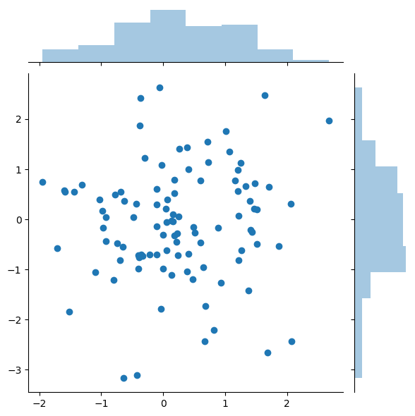                  

Every bit you lot can run into we are also getting the distribution plot for the ten and y value.

Bubble plot

A bubble plot is a scatterplot where a third dimension is added: the value of an boosted variable is represented through the size of the dots.

You demand to add another command in the scatter plot s which represents the size of the points.

          # Bubble Plot. The size of            points            changes based on a            third            varible. x =            np.random.rand(100) y =            np.random.rand(100) s =            np.random.rand(100)*200            plt.scatter(x, y, due south=southward,colour='red') plt.show()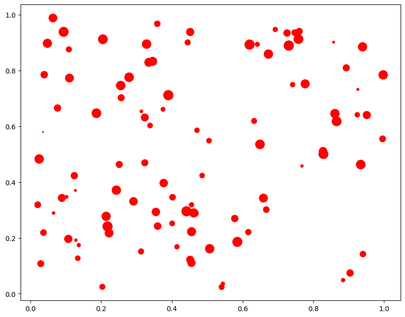                  

The size of the bubble represents the value of the 3rd dimesnsion, if the chimera size is more then it ways that the value of z is large at that betoken.

Exploratory Analysis of mtcars Dataset

mtcars dataset contains the mileage and vehicle specifications of multiple automobile models. The dataset tin can be downloaded here.

The objective of the exploratory analysis is to sympathise the relationship between the various vehicle specifications and mileage.

                      df=pd.read_csv("mtcars.csv") df.head()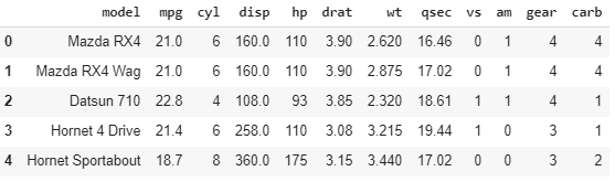                  

Yous can see that the dataset contains different informations well-nigh a car.

First permit'south see a scatter plot to see a distribution between mpg and disp and their histogramic distribution. You can do this past using the jointplot() role in seaborn.

          #            articulation            plot            for            finding distribution sns.jointplot(x=df["mpg"], y=df["disp"],color='red', kind='scatter')                  

          <seaborn.axisgrid            .JointGrid            at            0x7fbf16fcc5f8>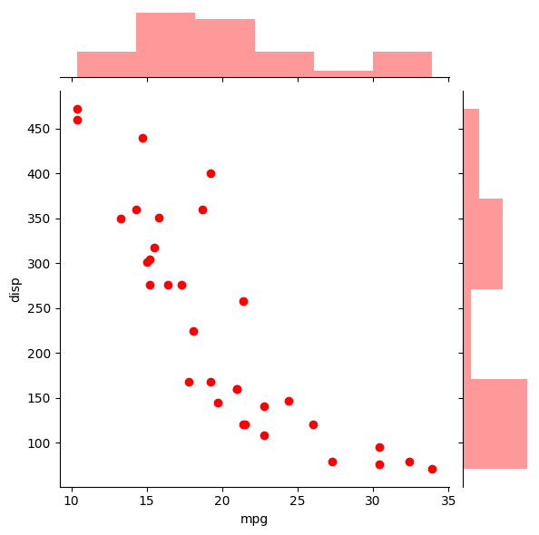                  

Multiple Line of best fits

If you demand to exercise linear regrssion fit for multiple categories of features between x and y, like in this case, I am further dividing the categories accodring to gear and trying to fit a linear line appropriately. For this, use the hue= argument in the lmplot() function.

          #            Linear            -            Line            of            best fit import seaborn            as            sns df=pd.read_csv('mtcars.csv') plt.rcParams.update({'figure.figsize':(10,8),            'figure.dpi':100}) sns.lmplot(x='mpg', y='disp',hue='gear', data=df);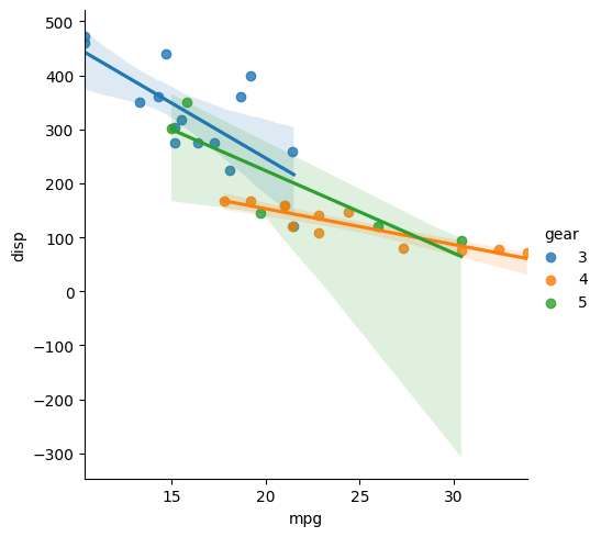                  

See that the function has fitted 3 different lines for iii categories of gears in the dataset.

Adjusting colour and style for different categories

I splitted the dataset according to dissimilar categories of gear. Then I plotted them separately using the besprinkle() function.

                      # Color and fashion change according to category            # Data            df=pd.read_csv('mtcars.csv') df1=df[df['gear']==3] df2=df[df['gear']==4] df3=df[df['gear']==v]            # PLOT            plt.besprinkle(df1['mpg'],df1['disp'],color='blue', marker=            '*',            characterization            ='gear=three')            plt.scatter(df2['mpg'],df2['disp'],colour=            'cherry-red', mark='v',            label            ='gear=four')            plt.besprinkle(df3['mpg'],df3['disp'],colour=            'green', mark='.',            label            ='gear=five')            plt.legend()                  

          <matplotlib.fable            .Legend            at            0x7fbf171b59b0>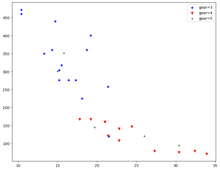                  

Text Annotation in Scatter Plot

If y'all need to add any text in your graph utilize the plt.text() function with the text and the coordinates where you demand to add the text as arguments.

          # Text annotation            in            besprinkle plot df=pd.read_csv('mtcars.csv') df1=df[df['gear']==3] df2=df[df['gear']==4] df3=df[df['gear']==5]  # Plot plt.scatter(df1['mpg'],df1['disp'],color='blue',            marking=            '*', characterization='gear=three') plt.scatter(df2['mpg'],df2['disp'],color=            'red',            mark='v', label='gear=four') plt.besprinkle(df3['mpg'],df3['disp'],color=            'green',            marker='.', characterization='gear=five') plt.legend()  # Text Annotate plt.text(21.five+0.ii,            255,            "gear=3", horizontalalignment='left',            size='medium',            color='blue', weight='semibold') plt.text(26+0.2,            120,            "gear=five", horizontalalignment='left',            size='medium',            colour='dark-green', weight='semibold') plt.text(24.5+0.2,            145,            "gear=4", horizontalalignment='left',            size='medium',            color='red', weight='semibold')                  

                                    Text              (24.7,                145,                'gear=4')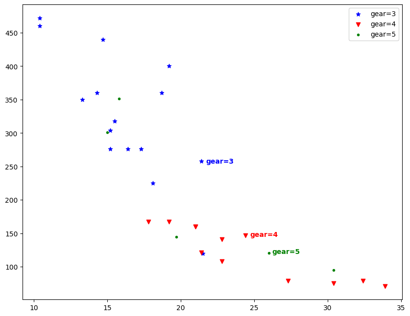                              

Bubble Plot with Categorical Variables

Usually you lot will use 2 varibales to plot a besprinkle graph(x and y), then I added another categorical variable df['carb'] which volition be implied by the colour of the points, I also added some other variable df['wt'] whose value will be unsaid co-ordinate to the intensity of each color.

                      # Bubble Plot            url =            'https://gist.githubusercontent.com/seankross/a412dfbd88b3db70b74b/raw/5f23f993cd87c283ce766e7ac6b329ee7cc2e1d1/mtcars.csv'            df=pd.read_csv(url)            # Plot            plt.scatter(df['mpg'],df['disp'],alpha =0.seven, s=100* df['wt'], c=df['carb'],cmap='plasma')            # Decorate            plt.xlabel('MPG') plt.ylabel('DISPLACEMENT'); plt.championship('Bubble Plot') plt.legend();                  

          No handles            with            labels found            to            put            in            legend.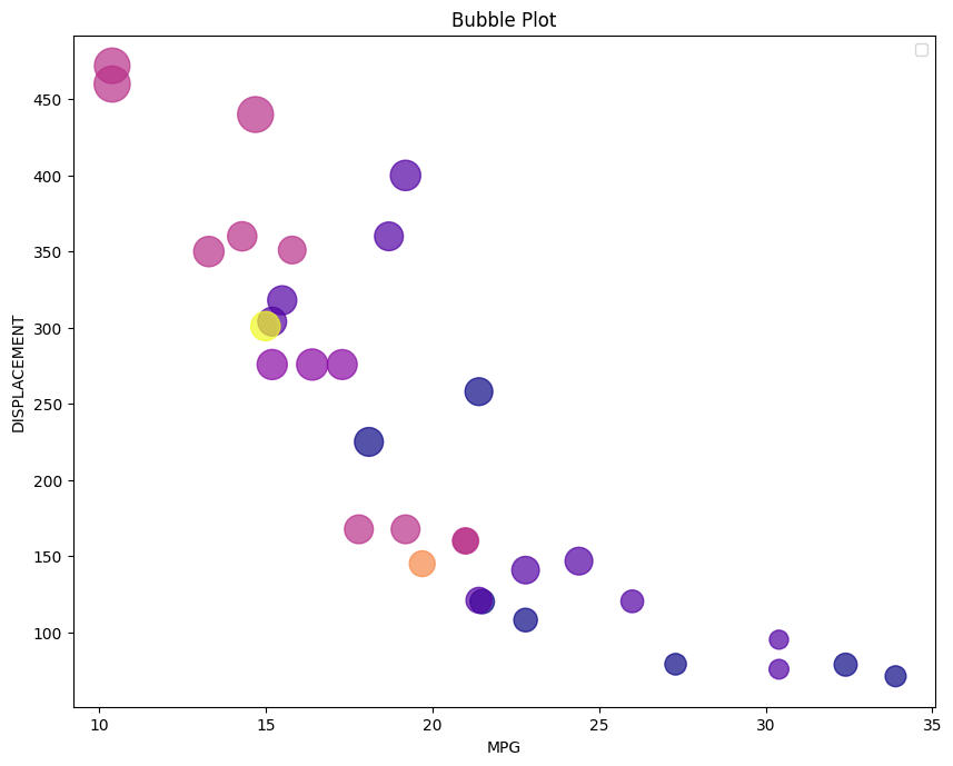                  

I have plotted the mpg value vs disp value and besides splitted them into different colors with respect of carbvalue and the size of each bubble represents the wt value.

alpha paramter is used to chage the color intensity of the plot. More the aplha more will be the color intensity.

Categorical Plot

                      # Chiselled Plot            sns.catplot(x="cyl", y="disp", hue="gear", kind="swarm", data=df); plt.title('Categorical            Plot')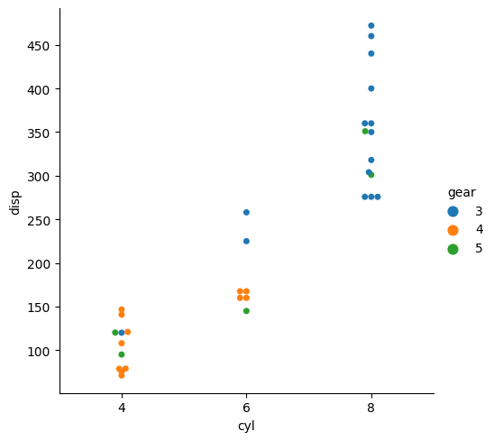                  

sns.catplot() is used to give admission to several axes-level functions that show the relationship betwixt a numerical and one or more than categorical variables using one of several visual representations.

Use the hue= command to further separate the information into another categories.

Recommended Posts

1. Top 50 Matplotlib Visualizations
2. Matplotlib Tutorial
3. Matplotlib Pyplot
4. Matplotlib Histogram
5. Bar Chart in Python
6. Box Chart in Python

camargoiont1964.blogspot.com

Source: https://www.machinelearningplus.com/plots/python-scatter-plot/

Share this post